Micro-Doppler time-frequency analysis

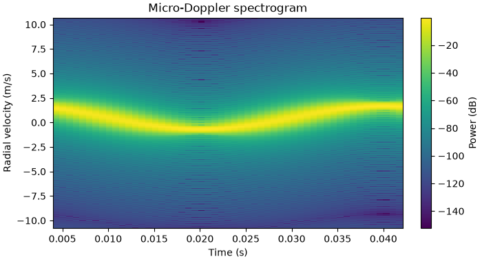
Resolve a sinusoidally varying radial velocity with a radar-aware STFT. The same result carries frequency, time, and velocity coordinates.

from __future__ import annotations

import numpy as np
from matplotlib import pyplot as plt

from pyradar.base import Radar
from pyradar.rsp import micro_doppler_spectrogram

radar = Radar.awr1843_rampcnn()
sampleRate = 1.0 / radar.slowTimeInterval
time = np.arange(512) / sampleRate
meanVelocity = 0.5
microVelocity = 1.2
motionFrequency = 25.0

# Doppler phase is the time integral of 2 v(t) / wavelength.
phaseCycles = (2.0 / radar.wavelength) * (
    meanVelocity * time
    + microVelocity
    * np.sin(2.0 * np.pi * motionFrequency * time)
    / (2.0 * np.pi * motionFrequency)
)
slowTimeSignal = np.exp(2j * np.pi * phaseCycles)
result = micro_doppler_spectrogram(
    slowTimeSignal,
    radar=radar,
    segmentLength=96,
    overlap=88,
    fftSize=256,
)

figure, axis = plt.subplots(figsize=(7, 3.8), constrained_layout=True)
powerDb = 10.0 * np.log10(np.maximum(result.power, np.finfo(float).tiny))
image = axis.pcolormesh(result.time, result.velocity, powerDb, shading="auto")
axis.set(
    xlabel="Time (s)",
    ylabel="Radial velocity (m/s)",
    title="Micro-Doppler spectrogram",
)
figure.colorbar(image, ax=axis, label="Power (dB)")
plt.show()